Colour Transport — Theory and the Stretch Fit
NebulaScope’s colour transport transfers the colour distribution of a reference image onto the displayed image. It has two application modes with very different data-integrity properties:
- Exact transport — pixels are rewritten through an empirical optimal transport map (a new list entry; the source is never modified).
- Stretch fit — no pixel is written at all: NebulaScope fits the display stretch so that the source looks like the transported result. Data loss is zero by construction.
This chapter derives both, and explains precisely why mode 1 can posterize and amplify noise, and why mode 2 cannot.
1. The distribution-transfer problem
Work in display space: each pixel of the source is a colour vector \(u \in [0,1]^3\) drawn from a distribution \(\mu_s\); the reference’s pixels follow \(\mu_r\). We seek a map \(T : [0,1]^3 \to [0,1]^3\) such that when \(u\) is distributed as \(\mu_s\), \(T(u)\) is distributed as \(\mu_r\) — written \(T_\# \mu_s = \mu_r\) (“\(T\) pushes \(\mu_s\) forward onto \(\mu_r\)”). Among all such maps, optimal transport selects the one moving colours the least, i.e. minimising \(\mathbb{E}\,\lVert T(u) - u \rVert^2\).
Alignment is irrelevant: only the two colour distributions matter, which is why the images need not overlap, match in size, or even show the same field.
1.1 One dimension is solved exactly
For scalar distributions with cumulative distribution functions \(F_s\) and \(F_r\), the optimal map is the classical monotone rearrangement
\[T = F_r^{-1} \circ F_s ,\]
i.e. the value at source quantile \(q\) maps to the reference value at the same quantile. This is exactly a histogram specification, and it is the unique monotone solution.
1.2 Sliced transport in three dimensions
In \(\mathbb{R}^3\) no closed form exists, but the 1-D solution can be sliced (Pitié et al.’s iterative distribution transfer, the same family as the sliced Wasserstein methods): repeat, for \(k = 1 \dots K\),
- draw a random rotation \(R_k \in SO(3)\);
- project both point clouds onto the three rotated axes;
- apply the 1-D monotone rearrangement independently along each axis;
- rotate back.
Each iteration reduces the discrepancy between the current and reference distributions; after \(K \approx 15\) sweeps the marginals agree along enough directions that the full 3-D distributions essentially match.
Implementation notes. NebulaScope estimates the maps from at most \(2 \times 10^5\) samples per image, restricted to each view’s visible region (off-screen features must not steer the match) and excluding near-saturated pixels (their colours are unmatchable). Each 1-D map is tabulated at 1024 quantile knots with linear interpolation between them, and the rotation sequence is deterministically seeded, so results are reproducible. A strength \(s \in [0,1]\) blends the result with the original: \(u' = u + s\,(T(u) - u)\). Mono image pairs skip the slicing and use the 1-D rearrangement directly.
2. Why exact transport degrades data
Two artefacts are inherent to pushing pixels through an empirical map — no implementation detail removes them entirely.
2.1 Posterization from tied samples
The empirical map is built from finite, quantized data. Where many samples share one value \(v\) (ties are guaranteed when the source was ever integer data), the empirical CDF jumps: the map sends the whole tie-run to a single output, and the next distinct input value lands a finite step away. The transported histogram develops gaps and spikes — visible as banding in smooth gradients. Iterating the slicing compounds the effect.
2.2 Noise amplification from map slope
For smooth densities \(f_s, f_r\), differentiating \(F_r(T(v)) = F_s(v)\) gives the local slope of the 1-D map:
\[T'(v) \;=\; \frac{f_s(v)}{f_r\!\big(T(v)\big)} .\]
Small perturbations (noise) scale by this slope: \(\sigma_\text{out} \approx T'(v)\,\sigma_\text{in}\). Wherever the reference distribution is locally thinner than the source — i.e. the reference has more contrast in that range, exactly what you asked for — \(T' > 1\) and the noise is stretched with the signal. Matching a punchy reference therefore necessarily amplifies background noise under any exact histogram match.
3. The stretch fit: match the look, not the pixels
NebulaScope’s display applies, per channel \(c\), a smooth parametric transfer to the raw value \(v\):
\[D_c(v) \;=\; \mathrm{MTF}\!\big(W_c(v);\, m_c\big),\]
where the window normalises and clips,
\[W_c(v) \;=\; \operatorname{clip}_{[0,1]} \left( \frac{\dfrac{v - \ell_c}{h_c - \ell_c} - b_c}{w_c - b_c} \right),\]
with data range \([\ell_c, h_c]\) and black/white points \(b_c, w_c\), and the midtone transfer function is the rational curve
\[\mathrm{MTF}(x; m) \;=\; \frac{(m-1)\,x}{(2m-1)\,x - m}, \qquad m_c = \frac{\mathrm{mid}_c - b_c}{w_c - b_c},\]
which fixes \(\mathrm{MTF}(0)=0\), \(\mathrm{MTF}(1)=1\) and \(\mathrm{MTF}(m)=\tfrac12\). Every such curve is smooth and strictly monotone on the window.
The fit. Let \(t_i = T_c(u_i)\) be the transported display values of a pixel sample and \(v_i\) the corresponding raw values. The stretch fit solves, independently per channel,
\[\min_{\,b_c,\ \mathrm{mid}_c,\ w_c}\; \sum_i \omega_i \Big( D_c(v_i;\, b_c, \mathrm{mid}_c, w_c) - t_i \Big)^{2}, \qquad \omega_i = 0.05 + t_i,\]
a bounded three-parameter weighted least-squares problem. The intensity weighting \(\omega_i\) matters: background pixels vastly outnumber signal pixels, and an unweighted fit would match the sky while shrugging at the nebula. Weighting each residual by the (floored) target brightness makes the signal colours govern the fit while the small floor keeps the black point anchored. Stars are best excluded at the source — match starless renditions of both images.
NebulaScope solves the per-channel problem by coordinate descent whose one-dimensional subproblems are golden-section line searches: black → white → midtone in turn, each over the full extended handle domain \([-1, 2]\) (one data span beyond each end — a black point below the data minimum is how a lifted reference floor is matched), sweeping until the objective stops improving (the black–white direction is a shallow valley, so the sweep count is adaptive rather than fixed), on up to \(6 \times 10^4\) sample pairs.
With the colour-mix stage on (the default), that per-channel fit is one block of an outer alternation. Cross-channel structure — a starless pair’s transport is almost purely a palette rotation — is outside any per-channel family, so a second block fits a full \(3\times 3\) colour mixer \(M\) on the curves’ output, by weighted least squares in closed form (one shared Gram-matrix inversion — exact, no search, no local minima). The two blocks alternate as a block coordinate descent: each round re-fits the curves against the mixer-inverted target, then re-solves the mixer; fitted sequentially instead, the least-squares escape is desaturation — the curves absorb a compromise the mixer can no longer undo. The root-mean-square residuals are reported in the status bar.
The result is only a stretch state: it lives in the same place as any Auto STF, composes with copy/paste and Apply to All, persists in the sidecar, and the underlying data is untouched.
3.1 Guarantees
- Zero data loss — nothing is written; the “result” is a view.
- No posterization — the fitted curve is smooth and strictly monotone; there are no empirical steps for ties to collapse onto.
- Controlled noise behaviour — the curve’s slope is the smooth parametric \(D_c'(v)\), free of the locally extreme slopes an empirical density ratio can produce.
3.2 Stage two: fitting the colour adjustments
Optionally, a second stage narrows the separability gap. With the fitted per-channel curves held fixed, NebulaScope fits the four cross-channel colour adjustments — temperature, tint, hue, saturation — minimising the intensity-weighted error over full RGB triples:
\[\min_{\theta}\; \sum_i \omega_i\, \big\lVert A_\theta\big(D(v_i)\big) - T(u_i) \big\rVert^2 ,\]
where \(A_\theta\) is the adjustment operator. These four parameters mix channels — which is precisely what OT’s slicing rotations do and what separable curves cannot — so hue-rotation targets that stage 1 misses become reachable. The status bar reports the overall RMSE after this stage; with undo one keystroke away, trying both variants costs nothing.
3.3 The approximation gap
The stretch family is separable: three independent monotone curves. The optimal transport map is generally not — its slicing rotations mix channels, which is how it can rotate hues. The projection of \(T\) onto the separable family therefore reproduces global colour balance and tonality closely, but cannot express hue rotation. The reported per-channel RMSE quantifies this gap for your pair of images; when it matters, the exact mode remains one checkbox away.
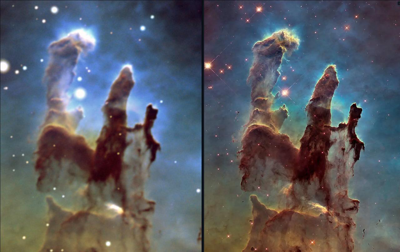
The thesis of this chapter, taken to its limit: the Pillars of Creation from a TEC 140/980 refractor at an amateur club’s remote observatory — about 10 h over two nights, session planned and operated by the author — matched (M) and colour-transported non-destructively toward the Hubble Space Telescope’s famous rendition (right; NASA/ESA/Hubble Heritage Team). The reference need not come from your data, your instrument, or even your planet: transport matches distributions, and what remains different after the match is optics and orbit, not processing.
Exactly how much optics-and-orbit remains is a measurable question — the PSF study appendix takes this very pair and measures it: the refractor’s true PSF from the extended structure, star-free, with Hubble as ground truth.
4. Practice
- Dialog: Tools ▸ Transport Colors from Reference…, tick Apply as stretch fit. Scripts:
transport <row> [strength%] stretch [colour]. Keep the colour-adjustment stage on for cross-palette matches: a starless pair’s transport is mostly a cross-channel rotation — the one thing per-channel curves cannot express (stars pin all three channels at the bright end, which is why starry pairs fit well without it). Both lossless options are on by default. - Strength applies before the fit — the fit targets the blended result.
- Framing is the relevance mask. Both distributions are estimated only from what is on screen: the source from the active view’s visible rectangle, the reference from its cell’s visible rectangle when it is displayed in one (rotations are unwound so expansion borders never contribute; saturated pixels ≥ 0.98 are dropped from both). When a calibrated Match has rotated a view’s navigation, the mask is the largest rectangle inside the visible quad — never its bounding box, whose off-screen sky would silently steer both distributions toward whatever surrounds the framed region. A reference that is only a list row — shown in no cell — is estimated from its whole image. So to control what the match is judged by, put the reference in a split cell and frame the region that matters: pan away from a gradient or a frame edge, and the transport never sees it.
- Both modes are undoable: the exact mode as a list-entry addition, the stretch fit as a stretch-state change (⌘Z restores the previous stretch).
- The fit absorbs the current display (including adjustments) into fresh Linear black/mid/white values and resets the adjustment sliders, so what you see immediately after is the fitted match itself.
- Judging RMSE: values are in display units on \([0,1]\); experience suggests a fit below \(\sim 0.02\) is visually convincing, while larger residuals usually indicate the reference demanded a hue rotation.
- The fit uses the whole handle domain. The fitted black and white points may lie outside the source’s data range — black below the minimum when the reference carries a lifted floor (a pedestal the source lacks), white above the maximum when the reference does not saturate where the source does. With the earlier \([0,1]\) bounds the source minimum always displayed as 0 and the fit paid for it in the shadows; the search now spans one data span beyond each end and iterates to convergence, so such references are matched at both ends.
- The reference need not show the same field. Transport matches distributions, never pixels, so any image with the same kind of content is a legitimate reference: two different parts of one supernova remnant (OIII and Hα ribbons on a starfield) have alike colour distributions even though no feature coincides. Field case: a collaborator’s NGC 6960 and NGC 6992, rendered with two different STFs, were made identical in colour from two JPEGs alone — no linear data, no pixel access, different fields. The non-destructive fit is what makes this safe: a monotone per-channel curve plus a global hue/saturation move cannot invent structure where the distributions genuinely disagree, so “make these alike” degrades gracefully to “as alike as a display transform can be”. And because the result is a display block (§6), the match is a file you can hand back.
5. Appendix: imported display functions and the Möbius rebase
When an XISF carries the producing application’s saved screen stretch (the DisplayFunction element — PixInsight’s STF), NebulaScope applies it on first view. One structural mismatch must be resolved: PI defines its STF on the normalized \([0,1]\) container, so its white point (typically \(h = 1\)) can sit at a windowed coordinate \(1/k\) — often \(80\)–\(300\times\) — beyond the actual data maximum, whereas every NebulaScope control (plot, handles, value boxes, colorbar) is parameterised on the data range. Imported verbatim, the white handle would sit \(1/k\) plot-widths off-screen.
The key structural fact. The midtone transfer function
\[\mathrm{MTF}(x; m) \;=\; \frac{(m-1)\,x}{(2m-1)\,x - m}\]
is a Möbius transformation fixing \(0\) and \(1\); conversely, the MTF family is exactly the set of monotone Möbius maps with those two fixed points — two constraints on a three-parameter group leave one degree of freedom, the pivot \(m\) (where the output is \(\tfrac12\)).
Restriction and renormalisation. Let \(D(t) = \mathrm{MTF}(t; m)\) be the imported curve on its own window, and let \(k \in (0,1)\) be the window coordinate of the data maximum. Restrict to the data and rescale so the data maximum displays as level \(S\):
\[g(t') \;=\; \frac{D(k\,t')}{D(k)}, \qquad t' \in [0,1].\]
Scaling the argument (\(t = k\,t'\)) is Möbius; dividing by the constant \(D(k)\) is Möbius; compositions of Möbius maps are Möbius — and by construction \(g(0)=0\), \(g(1)=1\). Hence \(g\) is again an MTF: the family is closed under restriction-and-renormalisation, which is why a closed form exists at all. Its pivot is recovered with the closed-form inverse
\[\mathrm{MTF}^{-1}(y; m) \;=\; \frac{m\,y}{(2m-1)\,y - m + 1}, \qquad m' \;=\; \frac{\mathrm{MTF}^{-1}\!\big(\tfrac{D(k)}{2};\, m\big)}{k}.\]
No fitting, no sampling, no approximation: the rebased curve equals the original over every value that exists in the data.
Colour: one common level. Rescaling each channel by its own endpoint \(D_c(k_c)\) would silently re-white-balance the image — undoing precisely the calibration (e.g. SPCC) the file records. NebulaScope therefore uses a single common level
\[S \;=\; \max_c D_c(k_c),\]
placing channel \(c\)’s new white at \(\mathrm{MTF}^{-1}(S;\, m_c)\): the brightest channel’s white lands exactly on its data maximum (all handles on-plot) and every displayed value divides by the same \(S\),
\[D'_c(v) \;=\; \frac{D_c(v)}{S}\quad \text{for all data } v,\]
so the inter-channel ratios — hue and calibrated colour balance — are preserved exactly. The only deviation from the producing application’s screen is a uniform brightness factor \(1/S\) (typically under \(10\%\)), monotone and channel-symmetric.
Background reading: Pitié, Kokaram & Dahyot 2007 (the iterative distribution transfer this implements); Rabin et al. 2012 for the sliced Wasserstein viewpoint — full citations in the References.
6. Appendix: the display block — an open, reproducible appearance format
Every stretch fit ends as numbers, and NebulaScope writes those numbers down. Save Annotations & Display stores the complete display state in the image’s sidecar (<image>_annotation.json) under a display key. The block is plain JSON with a stated schema, every field maps to a closed-form equation in this book, and a standalone reference implementation (tools/render_sidecar.py, NumPy only, no NebulaScope code) reproduces NebulaScope’s rendering from it — verified in CI to a few float32 ULPs at every pixel (tests/conformance/). This is what makes a stretch explainable (read the block, know exactly what was done) and reproducible in other software (implement six short equations).
6.1 The block
"display": {
  "schema": 1,
  "fn": "ghs",                       // linear | log | asinh | ghs
  "count": 3,                        // channels the state was made for
  "channels": [                      // R, G, B (index 0 used for mono)
    { "lo": 0.0012, "hi": 0.9840,    // data window (raw units)
      "black": 0.031, "mid": 0.118, "white": 1.0 },   // normalized in [lo,hi]
    { ... }, { ... }
  ],
  "ghs":    { "D": 1.6, "b": 6.0, "SP": 0.18, "LP": 0.0, "HP": 1.0 },
  "cmap": "gray", "cmapInvert": false, "cmapSplit": false, "split": 0.25,
  "adjust": { "blackpoint": 0, "whitepoint": 1, "shadows": 0,
              "highlights": 0, "brightness": 0, "contrast": 0, "gamma": 1,
              "temperature": 0, "tint": 0, "hue": 0,
              "saturation": 0, "vibrance": 0,
              "mix": [1,0,0, 0,1,0, 0,0,1] }   // schema 2, optional
}
schema is the version of this block (independent of the sidecar’s own version); a reader must refuse a schema newer than it knows. Schema 2 adds one optional field, adjust.mix: a row-major 3×3 colour mixer applied FIRST in the colour stage, \(\mathbf{c}' = M\,\mathbf{c}\) — absent means identity, and a writer stamps schema: 2 only when the mix is present, so mixer-free blocks stay valid schema 1. The mixer is what the lossless colour-transport fit stores: temperature, tint, hue rotation and saturation are all linear in RGB, so a full matrix subsumes them, and it is the part a starless pair’s palette rotation needs. Enumerations are stored as names, never integers. black/mid/white and the GHS SP/LP/HP are normalized window coordinates and may lie outside \([0,1]\) (a black point below the data minimum, a symmetry point beyond the window): the pipeline below is defined for any real values, and a conforming implementation must not clamp them.
6.2 The pipeline, per channel \(c\) and raw pixel value \(v\)
Window. The channel’s black/mid/white handles live in normalized window coordinates on \([\mathrm{lo}_c, \mathrm{hi}_c]\) — that is what makes a state portable across images with different data ranges:
\[t \;=\; \operatorname{clamp}_{[0,1]}\!\left( \frac{\dfrac{v-\mathrm{lo}_c}{\mathrm{hi}_c-\mathrm{lo}_c} - \mathrm{black}_c} {\mathrm{white}_c-\mathrm{black}_c}\right).\]
Transfer \(T(t)\), one of:
linear,log,asinh— a base shape followed by the midtones transfer function (§5) with pivot \(m_c = (\mathrm{mid}_c-\mathrm{black}_c)/(\mathrm{white}_c-\mathrm{black}_c)\), clamped to \([0.001, 0.999]\): \[T(t) = \mathrm{MTF}\big(s(t);\, m_c\big),\qquad s(t) = \begin{cases} t & \text{linear}\\ \ln(1+500t)/\ln 501 & \text{log}\\ \operatorname{asinh}(50t)/\operatorname{asinh}50 & \text{asinh}\end{cases}\]ghs— one master curve shared by all channels: the normalized cumulative integral of the local-stretch slope \[\sigma(x) = D_e\,\big(1 + b\,D_e\,|x-\mathrm{SP}|\big)^{-(1+1/b)} \quad (b>0;\ \text{logarithmic } D_e/(1+|b|D_e|x-\mathrm{SP}|) \text{ for } b<0,\ \text{exponential } D_e e^{-D_e|x-\mathrm{SP}|} \text{ for } b=0),\] with \(D_e = e^{D}-1\) and \(x\) clamped to \([\mathrm{LP},\mathrm{HP}]\) before evaluating \(\sigma\) (linear protection zones); \(T(t) = \int_0^t \sigma \,/\, \int_0^1 \sigma\). NebulaScope evaluates this on a 4096-point trapezoid grid, and interpolates linearly between grid points; a conforming implementation does the same, which is what gives ULP-level agreement rather than mere visual agreement.
Tone adjustments (monotone, per channel, composed into \(T\)), in this order: black/white-point re-window, then \(y \mathrel{+}= \mathrm{shadows}\cdot 2y(1-y)^2\), \(y \mathrel{+}= \mathrm{highlights}\cdot 2y^2(1-y)\), \(y \mathrel{+}= \mathrm{brightness}/2\), \(y = \tfrac12 + (y-\tfrac12)\tan\!\big((\mathrm{contrast}+1)\tfrac{\pi}{4}\big)\), clamp, then \(y^{1/\gamma}\).
Colour adjustments (cross-channel, RGB only), in this order: the mix matrix (schema 2; identity when absent); white-balance gains \(R\,(1+0.30\,\mathrm{temp}+0.15\,\mathrm{tint}),\;
G\,(1-0.30\,\mathrm{tint}),\;
B\,(1-0.30\,\mathrm{temp}+0.15\,\mathrm{tint})\); the standard luminance-preserving hue-rotation matrix (the SVG/CSS hue-rotate coefficients) by hue degrees; then saturation about Rec.,709 luma \(Y\): \(C = Y + (C-Y)\,f\) with \(f = (1+\mathrm{saturation})\,(1+\mathrm{vibrance}\,(1-s))\), \(s\) the pixel’s HSV saturation. Clamp to \([0,1]\).
Output. The result is the Float32 [0,1] rendition (what Save Stretched As… bakes). The 8-bit screen image is this rounded to 255 levels — NebulaScope adds a ±1 LSB triangular dither on screen, which is a display cosmetic and deliberately not part of the format.
6.3 Reading a transport fit
A non-destructive transport fit (§3) is nothing but a display block: the per-channel black/mid/white it solved for, plus, when colour fitting was on, the adjust vector. Two fits diff as JSON, and the diff localizes where the effort went — windowing versus hue versus saturation — which is information about how the two images differ, not just a recipe.
6.4 Scope and non-goals of the reference implementation
render_sidecar.py covers the four transfer functions, per-channel windowing, all tone and colour adjustments, mono and RGB. False-colour maps (cmap other than gray, or the invert/split modifiers) are 8-bit tables defined by control points in src/core/Colormap.cpp, which remains authoritative for them; a mono image with an active map renders through the same stretch and is then indexed into that table.